Generate Vision Proprioception Data for Deformable Objects


In this tutorial, we will demonstrate how PolyFEM can be used to generate vision proprioception data for soft robotics study. The GitHub repo of this tutorial can be found here.
Prerequisites
The following, items are necessary to complete this tutorial. To replicate the experiment, readers can use either the given mesh files or their own mesh files.
In this tutorial, we assume that readers already have PolyFEM installed. If not, the PolyFEM install instruction can be found here.
Meshes
To decrease the computing complexity of this tutorial example, we assume that the target item is the only deformable solid and the environment is rigid and immovable.
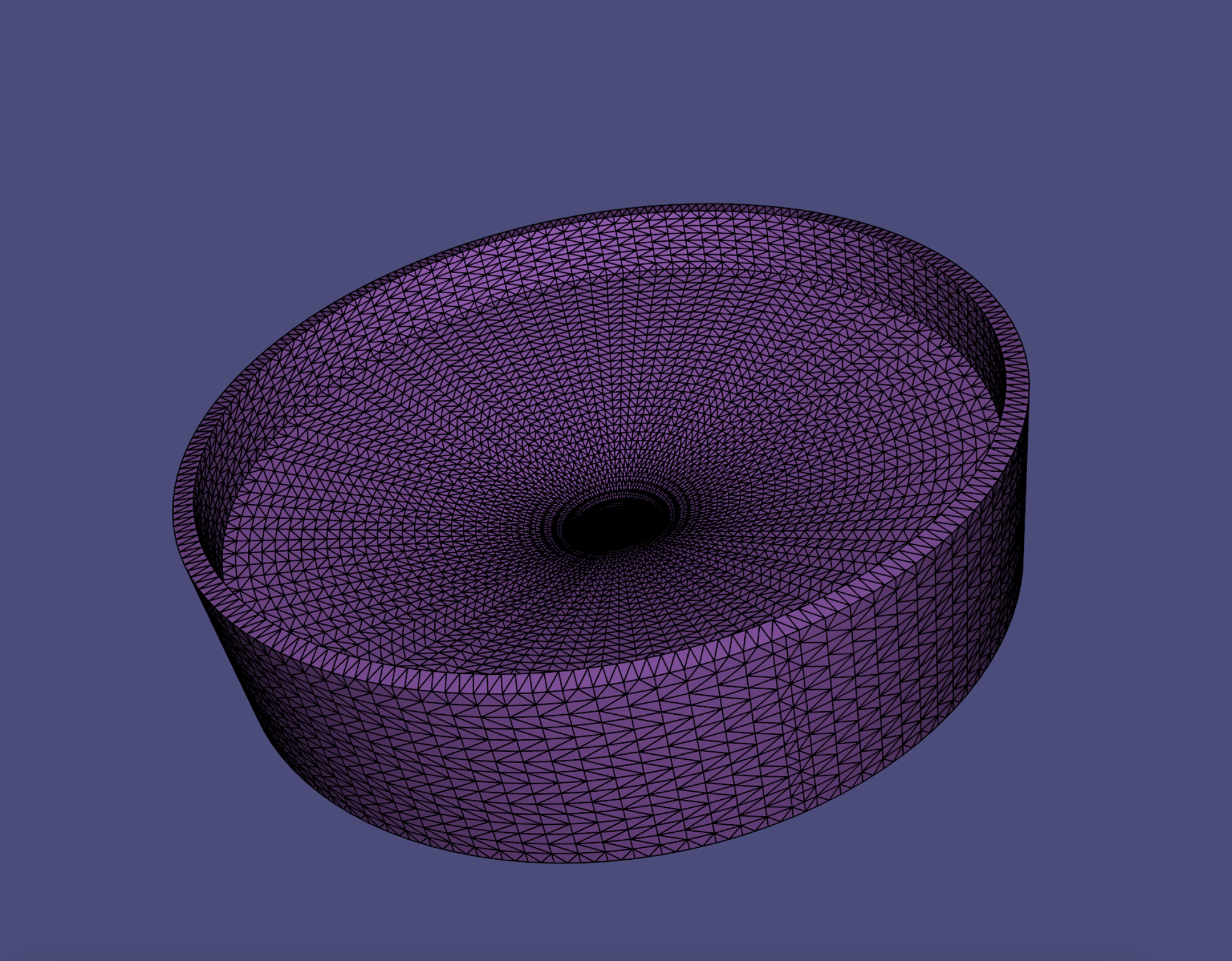
| Target Object Mesh (Radius: 0.5) | Environment Mesh (Radius: 5.0) |
|---|---|
 |
 |
Problem Formulation
This tutorial’s objective is to launch a deformable target object into an environment mesh (i.e. a sphere rolling in a bowl) and gather the corresponding vision-based proprioceptive data (the internal view that shows deformation). Such data can be utilized to investigate the relationship between vision-based proprioception and kinematics of deformable objects.
JSON Interface
PolyFEM provides an interface through JSON and Python. Here we demonstrate the JSON interface setup first. For more details, please refer to the JSON API.
Setup Similation
In this section, we will go over the JSON script that defines the simulation section by section. The complete JSON file can be found here.
Geometry
The "geometry" section specifies all geometry data required for simulation. For example, "mesh" defines the path to the volumetric mesh file. Then, the term "transformation" defines the operations that will be applied to the current mesh file. Next, volume selection specifies the mesh’s identifier, allowing other parameters to be applied to specific meshes based on volume selection.
Furthermore, is obstacle permits the definition of a mesh as part of the environment. Obstacles are fully prescribed objects and as such, only their surface needs to be specified.
json
"geometry": [{
    "mesh": "../data/sphere.msh",
    "transformation": {
        "translation": [-0.4, 0.18, 0],
        "scale": 0.1
    },
    "volume_selection": 1
}, {
    "mesh": "../data/scene_bowl.msh",
    "is_obstacle": true,
    "enabled": true,
    "transformation": {
        "translation": [0, 0, 0],
        "scale": 0.01
    }
}]
Mesh Related Configuration
In the previous section, we defined the simulation-required geometry. Following that, we must define their material properties and initial conditions. In the "initial_conditions" section, we assign the mesh with volume selection value 1 and an initial velocity of [2, 0, 2]. Next, in the materials section, we use NeoHookean for non-linear elasticity and define Young’s modulus E, Poisson’s ratio nu, and density rho.
Next, we define time step size as dt and time steps as the number of steps. enable in the contact determines whether collision detection and friction calculation are considered. And boundary conditions permit us to add gravity to the simulation with ease.
json
{
    "initial_conditions": {
        "velocity": [
            {
                "id": 1,
                "value": [2, 0, 2]
            }
        ]
    },
    "materials": [
        {
            "id": 1,
            "E": 5000.0,
            "nu": 0.3,
            "rho": 100,
            "type": "NeoHookean"
        }
    ],
    "time": {
        "t0": 0,
        "dt": 0.1,
        "time_steps": 100
    },
    "contact": {
        "enabled": true,
        "dhat": 0.0001,
        "epsv": 0.004,
        "friction_coefficient": 0.3
    },
    "boundary_conditions": {
        "rhs": [0, 9.81, 0]
    }
}
Simulation Related Configuration
json
{
    "solver": {
        "linear": {
            "solver": "Eigen::CholmodSupernodalLLT"
        },
        "nonlinear": {
            "line_search": {
                "method": "backtracking"
            },
            "grad_norm": 0.001,
            "use_grad_norm": false
        },
        "contact": {
            "friction_iterations": 20,
            "CCD": {
                "broad_phase": "STQ"
            }
        }
    },
    "output": {
        "json": "results.json",
        "paraview": {
            "file_name": "output.pvd",
            "options": {
                "material": true,
                "body_ids": true
            },
            "vismesh_rel_area": 10000000
        },
        "advanced": {
            "save_solve_sequence_debug": false,
            "save_time_sequence": true
        }
    }
}
Run Simulation
To run the simulation, the following command can be used where polyfem should be replaced with .../polyfem/build/PolyFEM_bin.
bash
cd PolyFEM_Tutorial_SoRo
mkdir output
polyfem --json json/scene_bowl.json --output_dir output
The simulation results will be output as a VTU file or a sequence of VTU files and a PVD file for the time sequence.
Python Interface
In addition, to the JSON files, PolyFEM also supports a Python interface through polyfem-python. More information can be found in the Python Documentation. Python interface not only allows to read configuration from JSON directly but also allows user to have more control during the simulation (eg. simulation stepping or change boundary conditions).
Import from JSON
If the JSON file is available, we can simply import the configuration by reading the JSON file.
```python import polyfem as pf
with open(‘./scene_bowl.json’) as f: config = json.load(f) solver = pf.Solver() solver.set_settings(json.dumps(config)) solver.load_mesh_from_settings() ```
Run Simulation in Python
Python interface provides a more flexible solution to simulate solving the time-dependent problem completely or interacting with the solver with steps.
```python
OPTION 1: solve the problem and extract the solution
solver.solve() pts, tris, velocity = solver.get_sampled_solution() ```
```python
OPTION 2: solve the problem with time steping
solver.init_timestepping(t0, dt) for i in range(timesteps): solver.step_in_time(t, dt, i) # interact with intermediate result ```
Visualize Simulation Results
To visualize the simulation sequential results in VTU format, we can use ParaView, an open-source, multi-platform data analysis and visualization application.
To view the results, please follow the instructions below.
![]paraview.png)
* Step 1: File - Open, select sequence group file step.vtu or step.vtm.
* Step 2: Click Apply under the tab Properties located on the left side of the GUI.
* Step 3: Click on Wrap By Vector to apply the displacement to the objects. This function can be found in the top menu bar.
* Step 4: Click again Apply under the tab Properties.
* Step 5: Now, the Play button can be used to view the time sequence results.
Bouns: Blender Rendering
Blender is a free and open-source 3D computer graphics software toolset that can be used for animation, rendering, and video games. Here, we are using Blender to create vision propriocetions (internal views). First, we need to convert the VTU outputs back to mesh files that represent the target object at each time step. Then, we can colorize the target object using vertex coloring and render the final image with the Blender camera instance.
Convert VTU to OBJ
To convert VTU to OBJ format, we can use the MeshIO library that is available in Python. A minimum example is shown below.
python
import meshio
m = meshio.read('step.vtu')
m.write('step.obj')
Colorize the OBJ Files
There are many different ways to colorize a mesh object. For example, coloring through mesh vertices, mesh faces, or a UV map. Here we demonstrate a simple way, which is to color the mesh using its vertices. The OBJ extension format support RGB floating values append to the vertex coordinates.
Blender Rendering using Python
In the example below, the Python script controls the rendering process. First, it loads colorized mesh files and adds light and camera to the pre-calculated position and orientation (based on the vertice coordinates and surface normal). It then renders the image using vertex color.
In this example, the camera is attched to one of the triangle in the surface mesh OBJ. And the camera is pointing at the center of the sphere, the rendering results are shown below.
blender_render.py:
```python
import os, sys
import math
import bpy
os.chdir(sys.path[0])
argv_offset = 0
IMPORT MESH
mesh = bpy.ops.import_mesh.ply(filepath=sys.argv[6+argv_offset]) mesh = bpy.context.active_object bpy.ops.object.mode_set(mode = ‘VERTEX_PAINT’)
ADD LIGHT
light_data = bpy.data.lights.new(‘light’, type=’POINT’) light = bpy.data.objects.new(‘light’, light_data) light.location = [float(sys.argv[8+argv_offset]), float(sys.argv[9+argv_offset]), float(sys.argv[10+argv_offset])] bpy.context.collection.objects.link(light)
ADD CAMERA
cam_data = bpy.data.cameras.new(‘camera’) cam = bpy.data.objects.new(‘camera’, cam_data) cam.location = [float(sys.argv[8+argv_offset]), float(sys.argv[9+argv_offset]), float(sys.argv[10+argv_offset])] cam.rotation_euler = [float(sys.argv[11+argv_offset]), float(sys.argv[12+argv_offset]), float(sys.argv[13+argv_offset])] cam.data.lens = 14 bpy.context.collection.objects.link(cam)
ADD MATERIAL
mat = bpy.data.materials.new(name=’Material’) mat.use_nodes=True
create two shortcuts for the nodes we need to connect
Principled BSDF
ps = mat.node_tree.nodes.get(‘Principled BSDF’)
Vertex Color
vc = mat.node_tree.nodes.new(“ShaderNodeVertexColor”) vc.location = (-300, 200) vc.label = ‘vc’
connect the nodes
mat.node_tree.links.new(vc.outputs[0], ps.inputs[0])
apply the material
mesh.data.materials.append(mat)
CREATE A SCENE
scene = bpy.context.scene scene.camera = cam scene.render.image_settings.file_format = ‘PNG’ scene.render.resolution_x = 512 scene.render.resolution_y = 512 scene.render.resolution_percentage = 100 scene.render.filepath = sys.argv[7+argv_offset]
RENDER
bpy.ops.render.render(write_still=1)
```
The rendering can be processed through Blender GUI or bash command as shown below.
bash
blender blender_project.blend -b --python blender_render.py -- target_mesh_path output_path camera_position_x camera_position_y camera_position_z camera_orientation_x camera_orientation_y camera_orientation_z