Sphere Pushing A Box
In this tutorial, we will be focusing on how to make an environment using a sphere to push a box on a table from scratch. In this scenario, one single JSON file for PolyFEM is seemingly not enough to simulate a varying and interactive environment like this. Therefore we will be using polyfempy, the python bindings for PolyFEM, to enable a more functional and versatile development.
Prerequisites
Install the Python Bindings of PolyFEM
In this tutorial, we are assuming you have already installed polyfempy in your machine. If not, please follow the instructions here. Note that there is no need to install standalone PolyFEM. All the dependencies that polyfempy requires will be installed automatically including PolyFEM. Also please note that please install and compile polyfempy from source by doing
python setup.py install
After installation, please try to run
python -c "import polyfempy as pf"
polyfempy is installed successfully.
Other Dependencies
Note that this tutorial is using a Conda virtual environment.
To build this project, there are some other depencies we need. Note that meshio and igl are optional. They are only required if you want to render the scenes with python.
- numpy:
conda install numpy - meshio (optional):
conda install -c conda-forge meshio - python bindings of libigl (optional):
conda install -c conda-forge igl
Data Preparation
The data needed in this tutorial can be found here. For triangle meshes, they are in surf_mesh folder and the volume meshes are in vol_mesh folder. The volume mesh files are all made using fTetWild. Feel free you make your own spheres and boxes.
All the codes and JSON files can be found here.
Environment with Volume Meshes
JSON Environment Setup
-
The first step is to make a JSON file
push_box_all_vol_mesh.jsonin the JSON folder for the initial setup with the sphere, cube, and the table in it. Let’s load the objects!The first mesh is the sphere, and the third one is the cube. Here, the cube’s mesh is re-scaled to act as the table. Feel free to use a 2D plane, or the mat mesh as the table in the GitHub repo.{ "geometry": [{ "mesh": "pushbox/assets/data/vol_mesh/sphere.msh", "transformation": { "translation": [-1.0, 0.2, 0], "scale": 0.1 }, "volume_selection": 1, "surface_selection": 1 }, { "mesh": "pushbox/assets/data/vol_mesh/cube.msh", "transformation": { "translation": [0, -0.0051, 0], "scale": [4, 0.01, 4] }, "volume_selection": 2, "surface_selection": 2, }, { "mesh": "pushbox/assets/data/vol_mesh/cube.msh", "transformation": { "translation": [-0.65, 0.2, 0], "scale": 0.4 }, "volume_selection": 3, "surface_selection": 3 }] } -
The second thing is to give proper material parameters to these objects.
The material parameters go to their matching meshes with the same{ "materials": [{ "id": 1, "E": 2e11, "nu": 0.3, "rho": 7750, "type": "NeoHookean" }, { "id": 2, "E": 2e11, "nu": 0.3, "rho": 7750, "type": "NeoHookean" }, { "id": 3, "E": 1e8, "nu": 0.48, "rho": 1500.0, "type": "NeoHookean" }], }"volume_selection"s. -
For the boudary conditions, we can set it as:
The first Dirichlet boundary condition with{ "boundary_conditions": { "rhs": [0, 9.81, 0], "dirichlet_boundary": [{ "id": 1, "value": ["0", "0", "0"] }, { "id": 2, "value": [0, 0, 0] }] } }"id":1is set for the sphere. They are set to["0", "0", "0"]just for initialization and the value of the boundary condition will be modified during the interaction.The second Dirichlet boundary condition is for the table since there’s no need for the table to move. That’s why it’s set to
[0,0,0].Note that there’s no Dirichlet boundary condition with
"id":3, however, the"boundary_id"for the cube is set to 3. This is because we want the cube to be completely free in all three dimensions.In addition to the Dirichlet boundary conditions, the problem should also be time-dependent and the gravity should also be specified in the
"rhs"argument (the gravity here is along the y-axis).
To view the whole JSON file, please go to pushbox_all_vol_mehses.json.
Python Environment Development
In this section, we will develop a python environment to control the sphere to interact with the box.
Class Initialization
In the src folder, create a python file pushbox.py. In this file, let’s first import necessary libraries and create a PushBox class with its __init__ function:
import polyfempy as pf
import json
import numpy as np

class PushBox:
    def __init__(self) -> None:
        self.asset_file = 'pushbox/assets/json/push_box_all_vol_mesh.json'
        with open(self.asset_file,'r') as f:
            self.config = json.load(f)
        self.step_count = 1
        self.solver = pf.Solver()
        self.solver.set_log_level(3)
        self.solver.set_settings(json.dumps(self.config))
        self.solver.load_mesh_from_settings()
        self.cumulative_action = np.zeros(3)
        self.dt = self.config["time"]['dt']
        self.t0 = self.config["time"]["t0"]
        self.solver.init_timestepping(self.t0, self.dt)

        self.id_to_mesh = {}
        self.id_to_position = {}
        self.id_to_vf = {}
        for mesh in self.config["geometry"]:
            if ("is_obstacle" in mesh.keys()) and (mesh["is_obstacle"]):
                self.obstacle_ids.append(mesh["surface_selection"])
            else:
                self.id_to_mesh[mesh["volume_selection"]] = mesh["mesh"]
                self.id_to_position[mesh["volume_selection"]] = mesh["transformation"]["translation"]
In the __init__ function, we load the environment configuration from the JSON file we just made, initialize a step counter and the polyfem solver. Here we set the log_level of PolyFEM to 3 which only displays the errors and warnings from PolyFEM. Feel free to change the log level to get more information or less based on docs for log_levels (More specifically, --log_level ENUM:value in {trace->0,debug->1,info->2,warning->3,error->4,critical->5,off->6} OR {0,1,2,3,4,5,6}).
One thing to mention is that polyfempy is always calculating the result for this time step based on the displacement from the initial position which is the position read from the JSON file. However, we only pay close attention to the action or movement we want to exert for this timestep, so self.cumulative_action would take care of previous displacements.
Take the action from the user
The solver is already initialized in the previous section, now we can design an interface for the users to pass new actions to the sphere from their side.
def set_boundary_conditions(self, action: np.ndarray): -> None
    t0 = self.t0 # starting time point for this timestep
    t1 = t0 + self.dt # end time point for this timestep
    self.solver.update_dirichlet_boundary(
            int(1), # the dirichlet boundary condition with id=1
            [
                f"{self.cumulative_action[0]} + ((t-{t0})*{action[0]})/({t1-t0})",
                f"{self.cumulative_action[1]} + ((t-{t0})*{action[1]})/({t1-t0})",
                f"{self.cumulative_action[2]} + ((t-{t0})*{action[2]})/({t1-t0})"
            ]
        )
        self.cumulative_action += action # accumulate the new action to displacement
This code block is to update the dirichlet boundary condition for the sphere in the next timestep. The current time is t0, and the current displacement is self.cumulative_action. Since the movement of the sphere needs to be continous and potential fatal penetration can happen if we just set the dirichlet boundary condition to self.cumulative_action + action. Image the action is large enough and greater than the edge length of the box while the sphere is on the left side of the box, then the sphere can teleport to the right side of the box without moving it. To avoid this kind of teleportation, we can interpolate the displacement from self.cumulative_action to self.cumulative_action + action for this timestep to make the movement of the sphere smooth and contiuous. The updated dirichlet boundary conditon in the above code block is the linear interplotion for the current timestep.
Run simulation for the current timestep
def run_simulation(self):
    self.solver.step_in_time(0, self.dt, self.step_count) # run simulation to the current time step, and the length of each timestep is self.dt
    self.step_count += 1 # increment the step counter
    self.t0 += self.dt # increment the starting time point for the next time step
To simulate the current timestep, we need to call self.solver.step_in_time, where the first argument of this function is the initial time of the simulation and the second argument is the time length for each time step and the third argument is the total time steps have been simulated now.
Get the position of each object
If you want to get the position information of each object in the simulation when you make interactions with the environment, you can get the positions of each mesh using this function.
def get_object_positions(self):
    points, tets, _, body_ids, displacement = self.solver.get_sampled_solution()
    self.id_to_position = {}
    self.id_to_vertex = {}
    for mesh_id, _ in self.id_to_mesh.items():
        vertex_position = points + displacement
        self.id_to_vertex[mesh_id] = vertex_position[body_ids[:,0]==mesh_id]
        mean_cell_id = np.mean(body_ids[tets], axis=1).astype(np.int32).flat
        tet_barycenter = np.mean(vertex_position[tets], axis=1)
        self.id_to_position[mesh_id] = np.mean(tet_barycenter[mean_cell_id == mesh_id], axis=0)
    return self.id_to_position
This function gets sample vertices for each mesh from the solver and these vertices are averaged to get a “centroid” of the object to represent its position.
Step function exposed to the user
def step(self, action: np.ndarray):
    self.set_boundary_conditions(action)
    self.run_simulation()
    return self.get_object_positions()
To view the implementation of the whole class, please go to pushbox.py.
Test of the Environment
Here’s a very simple but weird test case:
from pushbox.src.pushbox import PushBox
import numpy as np

env = PushBox()

# push forward
for i in range(5):
    action = np.array([0.1,0,0])
    env.step(action)

# go around the box
action = np.array([-0.1,0,0])
env.step(action)
action = np.array([0,0,0.3])
env.step(action)
action = np.array([1.0,0,0])
env.step(action)
action = np.array([0,0.3,0])
env.step(action)
action = np.array([0,0,-0.6])
env.step(action)
action = np.array([0,-0.4,0])
env.step(action)
action = np.array([0,0,0.4])
env.step(action)
You can create a test.py file for this, and run it in the project folder:
python test.py
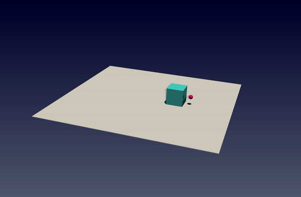
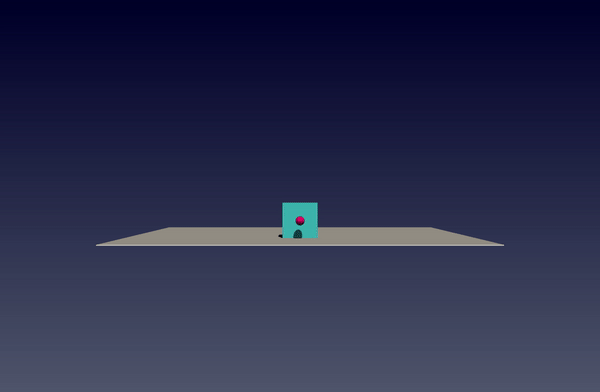
The result should be like the gifs at the beginning.
Environment with Triangular Meshes
In the previous environment, all the meshes are volume meshes, so the sphere, box, and table are all deformable. The ability of deformation for all meshes is generally not good (if you want three of them to be deformable, then you can skip the rest of the tutorial) and takes a long time to simulate. Thus in this section, considering the table is only a support base and the sphere is only an actuator, the table and the sphere can be rigid. Then we can set them as obstacles (a special type of mesh whose displacement is fully prescribed and need not be volumetric).
Json Environment Setup
Now the mesh part only needs to load the box and the sphere and the table can be loaded as obstacles:
{
    "geometry": [{
        "mesh": "pushbox/assets/data/vol_mesh/cube.msh",
        "transformation": {
            "translation": [-0.65, 0.2, 0],
            "scale": 0.4
        },
        "volume_selection": 3,
        "surface_selection": 3,
        "advanced": {
            "normalize_mesh": false
        }
    }, {
        "mesh": "pushbox/assets/data/surf_mesh/sphere.obj",
        "is_obstacle": true,
        "enabled": true,
        "transformation": {
            "translation": [-1.0, 0.2, 0],
            "scale": 0.1
        },
        "surface_selection": 1000
    }, {
        "mesh": "pushbox/assets/data/surf_mesh/cube_dense.obj",
        "is_obstacle": true,
        "enabled": true,
        "transformation": {
            "translation": [0, -0.0051, 0],
            "scale": [4, 0.01, 4]
        },
        "surface_selection": 1001
    }]
}
Note that the obstacles have no boundary conditions or material parameters (since they are already rigid) but only displacements. Also, there’s no need for Dirichlet boundary conditions anymore since the sphere is controlled by its displacement field.
The json file can be found at pushbox.json.
Python Environment Development
Class Initialization
In the src folder, create a python file pushbox_with_obstacles.py. The __init__ function stays the same except for the JSON file path.
Take the action from the user
def set_boundary_conditions(self, action):
    t0 = self.t0
    t1 = t0 + self.dt
    self.solver.update_obstacle_displacement(
            int(0),
            [
                f"{self.cumulative_action[0]} + ((t-{t0})*{action[0]})/({t1-t0})",
                f"{self.cumulative_action[1]} + ((t-{t0})*{action[1]})/({t1-t0})",
                f"{self.cumulative_action[2]} + ((t-{t0})*{action[2]})/({t1-t0})"
            ]
        )
    self.cumulative_action += action
Note that the obstacles have no ID fields, thus we can’t update its displacement with its id but the order of the obstacles in the JSON file. The index starts from 0. The rest part remains the same.
To view the whole implementation of the environment with obstacles, please go to pushbox_with_obstacles.py.
Test of the Environment
The test script remains the same except for the first import. Make sure to import PushBox from the correct file.
from pushbox.src.pushbox_with_obstacles import PushBox
The entire script can be viewed in test_with_obs.py.
This is the end of the tutorial. Enjoy!